
6. Application of ecosystem service framework in integrated planning: “LIFE Viva Grass Tool” example
6.1. Integrated planning approaches and tools
During the past decade, many tools and frameworks offering integrated planning approaches incorporating the concept of ecosystem services (ES) have been developed (Brown et al., 2018). Before exploring the details of these type of planning tools, and particularly the tools developed within the “LIFE Viva Grass” project, it is necessary to establish a common understanding of the concept of „integration“. Integration may refer to the inclusion of several disciplines and approaches in one single assessment (i.e the incorporation of socioeconomic information in ecosystem condition and ES assessments). Integration can also be understood as the structured combination of several ES mapping and assessment methodologies in one single Toolset (i.e. the combination of biophysical, social and economic mapping and assessment methods).
The inclusion of ES in spatial, landscape and environmental planning is recently increasing. Although this process is challenging due to the rigid structure of national spatial and landscape planning frameworks, many benefits arise from the integration of ES in planning processes. The communicative strength of ES enhances the inclusion of public stakeholders into planning processes and improves the understanding of public benefits of certain planning approaches. Moreover, ES help visualize the full spectrum of impacts and benefits of different (and often contrasting) planning scenarios.
Many of the existing spatial, landscape and environmental planning frameworks do not easily accommodate the concept of ES. For this reason, it is often necessary to develop tools that help instrumentalize the above mentioned integration. Many of these tools are flexible in terms of area, ES analyzed and data needs, but often require the end user to provide the base data and maps (i.e. InVEST). Other tools have a stronger focus in a specific area or particular planning issue and already contain pre-defined datasets (i.e. Nature Value Explorer).
The following sections outline the design, content and functionalities of the “Integrated Planning Tool” developed within the “LIFE Viva Grass” project.
6.2.”Viva Grass Integrated Planning Tool”
The “LIFE Viva Grass” project was launched in 2014, involving researchers and practitioners from the Baltic countries – Lithuania, Latvia and Estonia, and aiming to support the maintenance of biodiversity and ecosystem services (ES) provided by grasslands, through encouraging ecosystem-based planning and economically viable grassland management. The major task of the project was to develop an “Integrated Planning Tool” (hereinafter called the “Viva Grass Tool”), which would provide spatially explicit decision support for landscape and spatial planning and sustainable grassland management.
The “Viva Grass Tool” is operationalizing the ecosystem service concept into decision making by linking biophysical data on agroecosystems (e.g. soil quality, relief, land use/habitat types) with estimates on the ES supply as well as socio-economic context. The tool is integrated into an online GIS working environment which allows users:
- to assess the supply potential and trade-offs of grassland ES in user-defined areas, as well as
- to develop ecosystem-based grassland management and planning scenarios.
The “Viva Grass tool” is tested in eight case study areas across the three Baltic States (two farms, four municipalities, two protected areas and one county), each of them having spatial and thematic scale, as well as different data availability.
Thus the “Viva Grass tool” demonstrates the applicability of ES related information at different planning scales and contexts, which requires a consistent but flexible approach.
One of the challenges integrated planning commonly meets is the need to adapt to different planning scenarios and contexts, as well as meeting the needs of different stakeholder groups Dunford et al. (2017). In this regard, the “Integrated Planning Tool” developed in “LIFE Viva Grass” faces the same challenges. In order to overcome the aforementioned problems, the structure of the “Viva Grass Integrated Planning Tool” follows the framework of the tiered approach (see Chapter 3). In a tiered system, methods and tools are combined in a sequential way, so that each consecutive tier entails an increase in data requirements, methodological complexity or both (Grêt-Regamey et al., 2015). In the “Viva Grass tool”, each tier encompasses different methods and answers different policy questions (Fig. 6.1). .

Figure 6.1. The tiered approach for grassland ES mapping and assessment in the Baltic States within the “LIFE Viva Grass” project.
Following the tiered approach the “Viva Grass tool” offers the three applications or Modules: “VivaGrass Viewer”, “VivaGrass Bio-Energy” and “ VivaGrass Planner”, each designed for different user groups and context of decision making. The “VivaGrass Viewer” is targeted to general public and farmers, providing an overview on ES supply within a selected area, depending on selected management practice. By using this Module farmers can decide on most suitable management model, which would increase the ES supply. The “VivaGrass Bio-Energy” demonstrates the potential for using the grass biomass as source for energy (e.g. heating), thus highlighting the value of one particular ES. The “VivaGrass Planner” module has restricted access – it is targeted to professional users, who could apply the ES information in the spatial planning process.
All the Modules are operating by using: i) basemap of land use and supporting natural conditions; ii) look-up table (matrix) of ES assessment and iii) resulting ES distribution maps. Furthermore the “Viva Grass tool” offers the spatial visualisation ES bundles and trade-offs as well as hotspot and coldspot areas, which provides an added value in the land-use planning.
In the sections below, each tool component is explained in details.
6.2.1. “Viva Grass” basemap
6.2.1.1. Basemap methodology
As outlined in Chapter 3, ES maps constitute the essential basis for ES assessments. With the help of ES maps, we can spatially locate the flow of ES, we can detect mismatches between ES supply and demand or locate factors exerting pressure on the supply of ES. ES supply maps can be built on the basis of landuse/landcover maps (LULC) that define the spatial units that provide ES (i.e. forest, crop, grassland). The first step in any ES mapping analysis is therefore the definition of a LULC that contains the Service Providing Areas (SPAs) (see Chapter 3).
“LIFE Viva Grass” project encompasses the three Baltic States and nine case study areas and consequently, the construction of a basemap faced large differences in data availability. European-scale maps such as CORINE land cover (Soukup et al., 2016) do not offer the level of spatial and thematic detail required to link, in a spatially explicit way, grassland classes with the ES they provide. On the other hand, the basic national LULC maps differ substantially from one country to the other in terms of their thematic scales. Therefore a common grassland typology was created in order to provide the basis for the ES mapping and assessment in “LIFE Viva Grass” Project.
Keeping in mind that the potential delivery of ES is determined by the interaction of natural attributes, comprising both biotic and abiotic components, and human inputs and management strategies (Smith et al., 2017), the grassland classes that constitute the “LIFE Viva Grass” basemap were defined according to two main factors:
- The underlying natural conditions: Two factors were selected as descriptors of the environmental conditions that underpin the provision of ES in the grasslands of the Baltic States: Land quality and slope. The concept of land quality is an integrated evaluation of fertility of soils used in the Baltic States land evaluation systems and is composed of several factors, e.g. soil texture, soil type, topography, stoniness, and level of cultivation. Land quality was subdivided in four groups:
- Low quality soils, are associated poor soils with sandy soil texture, high risk of erosion, low capacity of nutrients supply and exchangeable elements and biological activity, very low estimated yields.
- Medium land quality soils, are associated with loamy sand soil texture, relatively low organic matter, low fertility, moderate capacity to accumulate nutrients and exchangeable elements.
- High land quality soils, are associated with loam and clay soil texture, moderate soil fertility, a high percentage of organic matter and capacity to accumulate nutrients and exchangeable elements.
- Hydromorphic soils, are soils developed on organogenic deposits, characterized by various soil fertility and relatively high rate of biological activity.
Slope was also included in underlying natural conditions: steeper slopes are associated with shallower soils with less water retention capacity due to gravity and with a higher risk for soil erosion and consequently affects the delivery of ES. The slope data was aggregated in three categories:
- plain surface (0 o – 4 o): no soil erosion
- gentle steepness (4 o – 10o): minimal soil erosion
- steep slope (>10 o): noteworthy soil erosion potential
- The management regime of the grasslands: One of the main driving factors for different supply potential of ES in grasslands is the intensity of management or level of interference in topsoil. Therefore, three types of grassland management regimes and one type of cropland were considered in the analysis as the foundation for creating the ES supply potential base-map:
- Cultivated grassland: Cultivated grasslands are seeded (often a monoculture – Festuca sp., Phleum sp., Dactylis sp.) and plowed, usually included in crop rotation and less than five years of age. Cutting of grass is done several (up to four) times a season. Fertilization is also a common practice to maintain high yields. Cultivated grasslands are associated with intensive farming systems.
- Permanent grassland: Permanent grasslands are generally defined as land used to grow grasses naturally or through cultivation which is older than five years. This type of grasslands are rarely seeded, contain both natural vegetation and cultivated species. Permanent grasslands are excluded from crop rotation, mostly used as hay fields and cut not more than two times a season or used as pastures. Permanent grasslands are associated with low input farming systems.
- Semi-natural grasslands: Semi-natural grasslands are the result of decades or centuries of low-intensity management and are currently not seeded or plowed. Semi-natural grasslands contain high levels of biodiversity (Bullock et al. 2011; Dengler and Rūsiņa 2012) and are used as low-intensity pastures or hay fields (one late cut per season), or solely managed to receive agri-environmental payments (Vinogradovs et al. 2018).
- Arable/cropland: Arable/cropland is defined as intensively managed farmland used for crop production, plowed at least one time in the season and usually fertilized.
The grassland classes alone do not account for the spatial dimension of ES. As pointed out by Walz et al. (2017), Service Providing Areas (SPAs) (see Chapter 3) constitute the best way to spatially capture the complex ecological systems that underlie the delivery of ecosystem services. SPAs can be defined as spatially delineated units that encompass entire ecosystems, their integral populations, and the underlying natural attributes. The unit used to define SPAs and map the potential delivery of grassland ES was the “basic agro-ecological unit” or field, which comprises the grasslands spatial configuration and boundaries. The basic agro-ecological unit is the smallest relevant unit to apply a management decision, defined as a continuous area with identical land-use.
Each of the abovementioned factors is represented by one spatial layer and were combined in a GIS environment through map algebra and GIS processing operations. Fig. 6.2 shows the classification of input variables and the data sources. As a result of this process, 30 grassland classes were obtained (Table 6.1). In addition to those, 10 arable land classes and 10 abandoned land classes were included in order to allow for the assessment of different LULC change scenarios. The SPAs generated in this process were used in the assessment of provisioning and regulating and maintenance ES.
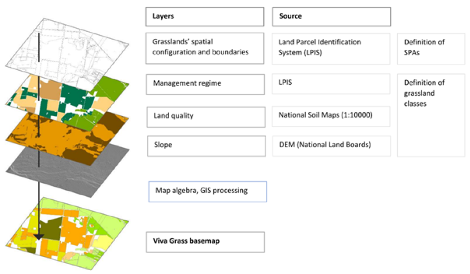
Figure 6.2. “LIFE Viva Grass” basemap workflow.
6.2.1.2. Look-up table based on expert knowledge (Tier 1)
The common grassland typology and map constitute the basis for the mapping and assessment of ES. Regarding the assessment of ES, at the most basic level, look-up tables based on expert estimates are used in Tier 1. Look-up tables provide the “Viva Grass Tool” with a qualitative assessment of ES supply, which is subsequently linked to the “Viva Grass” basemap and presented in an interactive way to the users of the “Viva Grass viewer” (see section 6.2.2). In addition, the ES scores contained in the look-up table are the basis for more complex analyses such as trade-offs, bundles and hot and coldspots (see following sections).
Within “LIFE Viva Grass”, the look-up table with expert-based scores was used exclusively to assess the supply of 13 ES belonging to the provisioning and regulating and maintenance categories. The ES supply assessment was organized in a three-step process:
- In the first step, the international experts panel selected a relevant set of ES provided by grasslands and one indicator per ES.
- In the second step experts individually score the provision of ES by the grassland classes based on a qualitative scale ranging from 0 (no relevant supply of the selected ES) to 5 (very high supply of the selected ES).
- In the third step, experts come to an agreement on the ES supply values in a series of focus group discussions (FGD). In each round of FGD, each expert contrasted his answers with the rest of the group and had the opportunity to re-score the ES.
A subset of the results of the ES assessment process are shown in Table 6.1.

Table 6.1. Extract of the look-up table based on expert estimates including grassland classes 21 to 30. A total of 30 grassland classes plus 10 arable land classes and 10 abandoned land classes were evaluated.
In order to visualize the supply of ES in a spatially explicit manner in the “Viva Grass Tool”, the results of the look-up table assessment are connected to the grassland classes defined in the basemap.
6.2.1.3. Trade-offs, bundles and hotspots (Tier 2)
A detailed explanation of the concepts of trade-offs, bundles and hotspots is provided in Chapter 4. In “LIFE Viva Grass”, the trade-offs, bundles and hotspots analyses constitute the core of Tier 2 and allow for a holistic evaluation of the impacts of management decisions and policies in multiple ES provided by grasslands. The results of these analyses are displayed in the “Viva Grass viewer” (section 6.2.2). The aim of displaying ES bundles in the “Viva Grass viewer” is to help the tool users to identify specific locations where several ES (bundles) are likely to respond similarly to different management options.
To find out how ES bundle together, a Principal Components Analysis was applied to the ES matrix. Similar analyses have been carried out by Depellegrin et al. (2016), Nikolaidou et al. (2017) and Zhang et al. (2017) among others.
The PCA revealed 3 main components which correspond to three bundles:
- Habitats bundle: 4 ecosystem services interact in this bundle: Herbs for medicine, pollination and seed dispersal, maintaining habitats and global climate regulation. The increase in one of the services in this bundle usually means an increase in the other two services. For example, in species rich grasslands, we are also likely to find a wide range of herbs with a medicinal value. Moreover, grassland management practices that aim to increase biodiversity, such us the reduction or complete elimination of plowing, and fertilization, also increase the carbon sequestration capacity of soils, which is a key service for the regulation of climate.
- Production bundle: This bundle is formed by 4 ecosystem services closely related to the productivity of ecosystems: Reared animals and their outputs, fodder, biomass for energy and cultivated crops. In this particular bundle, the underlying ecosystem function that drives the production of the four ES is the net primary production, or biomass production. Therefore, the increase in one of the services in this bundle usually means an increase in the other two services. However, biomass for energy not only depends on the productivity of grasslands, but also on the calorific potential of grassland species. At the same time, it shall be noted, that even the potential of the four services is based on the same underlying function – productivity, the actual use of ES can exclude each other (i.e. biomass for energy and cultivated crop production can exclude grazing or fodder production)
- Soils bundle: The 5 ecosystem services that form this bundle are related with the role of soil functions in ecosystem processes: Control of erosion rates, chemical condition of fresh waters, bio-remediation, filtration/storage/accumulation by ecosystems and weathering processes-soil fertility.The increase in one of the services in this bundle usually means an increase in the other two services.
Beyond simply identifying ES bundles, it is important to visualise their spatial configuration in order to incorporate the concept into planning processes. In “LIFE Viva Grass”, a grassland was mapped as belonging to a certain bundle if all ES in the bundle in that particular grassland scored above average (2.5) (Fig. 6.3). The analysis of bundle overlap reveals certain tradeoffs, for instance, intensification of agriculture, i.e. changing grassland maintenance practice in the same underlying biophysical conditions, will alter services in the “production” bundle and decrease ES in the “habitat” bundle. The direct driver behind tradeoff in grasslands is the management regime, that is, the human factor, the only factor that can be affected through planning decisions.
Results of cold/hot spot analysis are provided in the “Viva Grass Viewer” and can give the user distinctive information on accountancy of ES supply potential in selected agro-ecosystems. Cold spot is a spatial unit that provides a great number of ecosystem services at low or very low values. Hotspot is a spatial unit that provides ES at high or very high values. The number of services with particular values of interest (low/high) were derived from the ES assessment matrix. Cold/hot spot analysis is strongly complementary to the analysis of tradeoffs. For example, the “coldest” areas did not contain any tradeoff, as both production associated ES and regulating ES displayed low values. Landscape planners should address cold spots as areas with conflicts between two or more landscape functions, which in agro-ecosystems can be described as inappropriate management practice in given natural conditions. Moderate cold spots mostly displayed one of the tradeoffs, and planning decisions should be based on these. “Hotspot” areas should draw attention of decision makers as well, because of high conservation value and high vulnerability. The “hottest” according to assessment presented in “Viva Grass Tool” also did not contain tradeoffs because of high values in both competing bundles of ES. The high vulnerability of these agro-ecosystems is associated with their capacity to deliver even higher production under intensive agriculture.
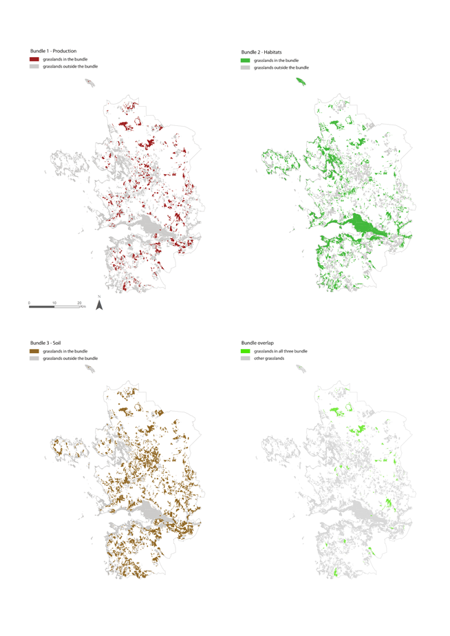
Figure 6.3. Grassland ES bundles in a Viva Grass pilot area: Lääne County (West Estonia).
6.2.2. “Viva Grass Viewer”
“Viva Grass Viewer” is basic module of the “Viva Grass Tool” accessible to general public, that aims to visualise the results of mapping and assessment of ES supply potential, as well the grouping of ES in bundles and interaction of ES in agro-ecosystems. “Viva Grass viewer” intents to serve informative and educational purposes, where user is able to get acquainted with ES approach, spatial distribution of the ES supply depending on underlying natural conditions and management practices. The Viewer is organized in representing exclusionary (one in the time) data layer or by using “swipe” or “double screen” options to simultaneously represent two contextual data layers. Contextual data layers available in “Viva Grass Viewer” are farmland land use, supply potential of selected ES, bundles and tradeoffs of ES supply potential, cold/hot spots of ES supply potential.
Default view (Fig. 6.4) of the Viewer is background map with land use data composed from IACS database, representing main classes of land use in agro-ecosystems: grasslands – semi-natural, permanent, cultivated and arable land. Additionally, where there is available data, abandoned farmland is shown.
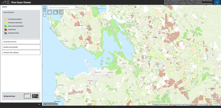
Figure 6.4. Default view Viva Grass Viewer – land use.
By clicking on land block of interest, user can view supply potential of ES in selected field. For informative and educational purposes user can change land use type to view changes in supply potential in case of land use change. Short descriptions and recommended maintenance practices where available are provided (Fig. 6.5).
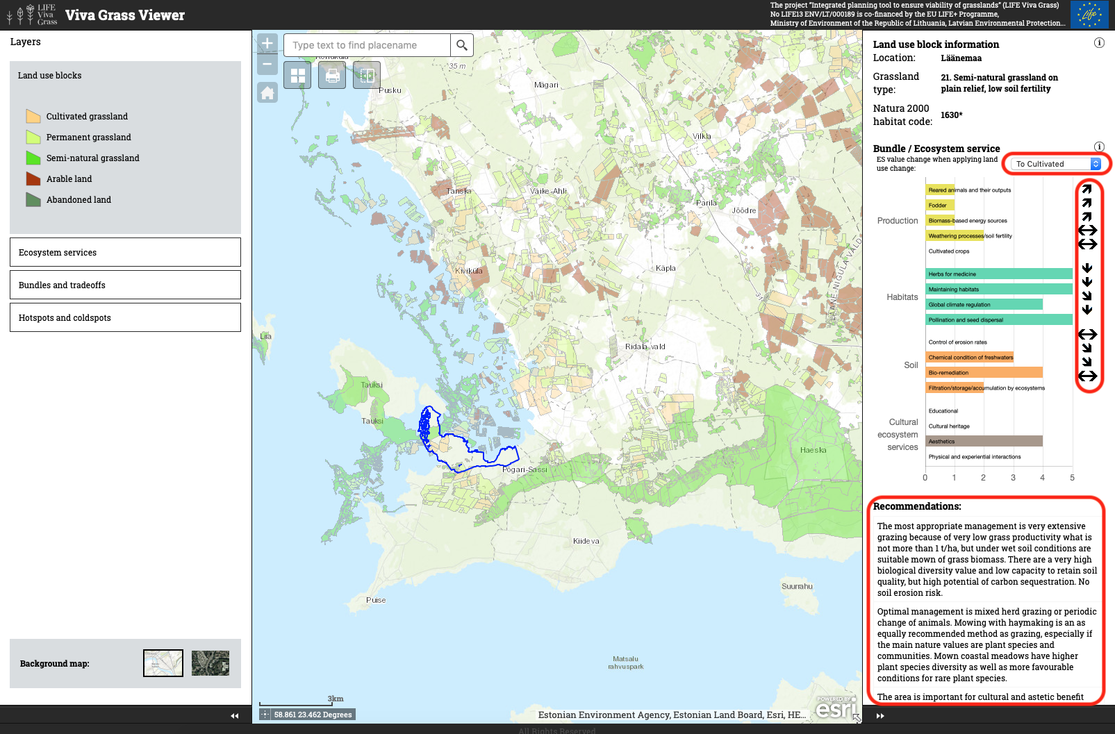
Figure 6.5. Land use change options.The user can change land use from the drop-down menu on the right side (e.g. from semi-natural grassland to cultivated as in the picture). The arrows show how it changes the provision of different ecosystem services. In the lower right corner the management recommendations for this particular grassland type are provided.
Supply potential of ES is the contextual data layer that allows user to explore mapping and assessment results of selected ES by choosing one in drop-down menu (Fig. 6.6). The theory and methodology of mapping and assessing ES supply potential is described in Chapter 3.
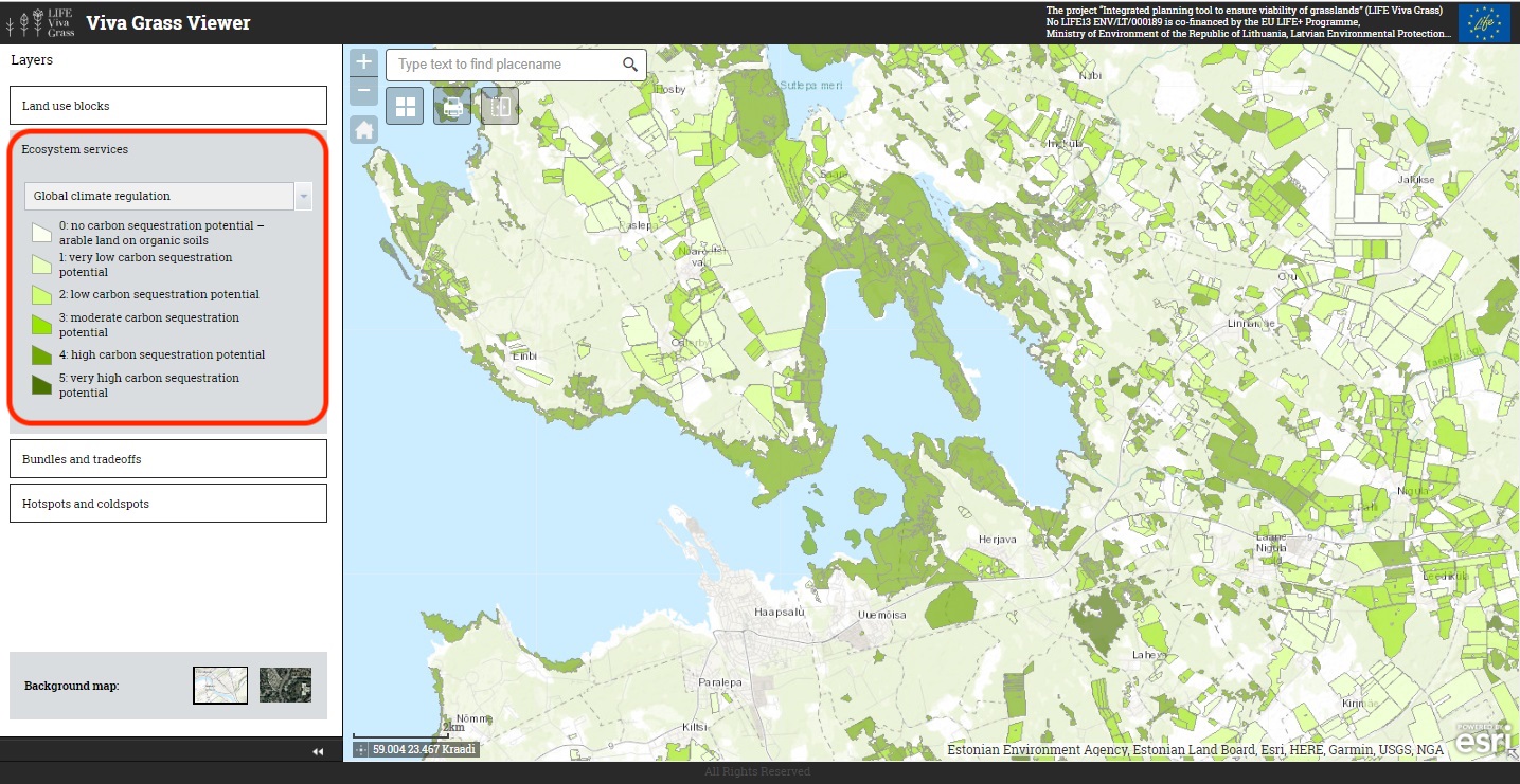
Figure 6.6. Supply potential of selected ES view and drop-down menu. By selecting certain ecosystem service from the drop-down menu on the left side, the user can see the provision (distribution and value) of this ecosystem service in different land blocks. The dark green colour shows higher provision of the selected ecosystem service.
Bundles and tradeoffs of ES supply potential is contextual data layer that represent spatial grouping and interactions of ES. User is able to explore those groupings and interactions by choosing one of them in drop-down menu (Fig. 6.7). Available selections are linked either to belonging to certain bundle or to having one of two possible tradeoffs. The theory and methodology of analysing interactions among ES is described in Chapter 4.

Figure 6.7. Bundles and tradeoff view and drop-down menu. Drop-down menu (left) enables to select different bundles (”Production”, ”Habitats”, ”Soils”) or trade-offs (in benefit of habitats or production). The green areas presented currently on the map belong to the “Habitats” bundle (grasslands important for preservation of biodiversity). By clicking on a concrete land plot, the detailed information about ecosystem services in that area will be displayed (on the right side).
Cold/hot spots of ES supply potential is contextual layer that represent the number of ES with either low or high values. User is able to explore different representations of cold/hot spots of ES supply potential by choosing one of it from drop-down menu (Fig. 6.8). Default choice is “cold/hot spots” – combined value from “number of ES with high values” and “number of ES with low values”. This selection gives general overview of territory in the context of its current potentiality to deliver ES. To get specific view on character of territory in context of shortages or abundance of ES supply potential, user can choose between additional selections – “Hotspots” or “Coldspots” – to view ranked ((1-5) values) combination of ES supply potential.

Figure 6.8. Cold/hotspots of ES supply potential and drop-down menu. In the marked “coldspot” area (the selected blue area) most of ecosystem services are provided at low or very low values, which can be also seen from the diagram of ecosystem services’ bundles on the right side.
To be able to simultaneously explore two contextual layers and view their spatial interactions on screen, user can choose either “swipe” tool, where it is possible to swipe between two layers on the same map extent (Fig. 6.9).
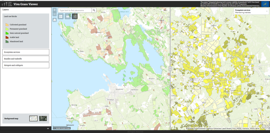
Figure 6.9. Swipe tool.
6.2.3 “Viva Grass Bioenergy”
The “LIFE Viva Grass BioEnergy” Module is developed as a tool for assessing grass-based energy resources (area, production, calorific potential for district heating) and informing relevant planners/stakeholders about areas with the highest potential for grass for energy (prioritizing).
Grasslands have a potential for energy production as solid biomass heating fuels. Whether grasslands are specifically cultivated for this purpose, or the grass mown from permanent and semi-natural meadows is used, grass can be burnt in co-fired plants for heat generation. In many cases, the use of grass bales for heating is a feasible alternative to regular biomass-based resources such as woodchips. Unused biomass resources resulting from semi-natural grassland management in some nature protection areas are left in the field and “wasted”.
The “Viva Grass BioEnergy” Module uses additional sources of information to enrich both the basemap and the ES assessment. The 10 semi-natural grassland classes (table 1) are updated with information about the Annex I habitat type they belong to. Subsequently, quantitative data collected from scientific literature sources is linked to the Annex I habitat types. The tool is therefore able to provide detailed information to the user about the average biomass production and average grass calorific power per semi-natural grassland type.
The “Viva Grass BioEnergy” module is accessible for everybody without registration and allows to select and summarize bioenergy potential from several grasslands. Additionally, the tool provides information on the current management status of the selected grasslands, as well as information about presence of reed encroachment and recommended grazing pressures per habitat type.

Figure 6.10. The “Viva Grass BioEnergy” module. Example from Matsalu National Park, Estonia. Reddish brown colours displayed in the map show the energy demand (GJ/year; based on number of inhabitants in block houses). Green colours show biomass potential (t/ha). The blue dot is existing district heating plant. The numbers on the right side show bioenergy demand (red, GJ/y), bioenergy calorific potential (yellow, GJ) and biomass potential (green, t) for the area selected by the user (currently the visible extent). From the drop-down menu on the left side it is possible to select also bioenergy potential, recommended grazing pressure or land use.
6.2.4. “Viva Grass Planner”
“Viva Grass Planner” is decision support system designed to operationalize ES concept for spatial planning. “Viva Grass Planer” is accessible for registered user; registration is carried out by system administrator.
“Viva Grass Planner” consists of two basic sub-modules, designed to carry out prioritization and classification functions and following representation of the results in map, as well the possibility to export processed data.
Prioritization is performed in following steps: choosing the criteria, weighting the criteria and displaying the results. Criteria can be selected out of available attributes consisting of the results of ES assessment (see Chapter 3) or from additional data added by user containing case specific attributes. To indicate relative importance of chosen criteria Tool user can assign weight ranging from 0-100%, so that the sum of all percentage would be equal 100% (Fig. 6.11). Weight of one component is calculated by calculating average value of normalized values and multiplying by user defined weight. Total weight of components should be 100%. Total weighted index is sum of selected components.
The resulting total weighted index can be further divided in priority categories. To create final prioritization of alternatives additional classification can be performed by employing supplementary data specified by the objective of enquiry.
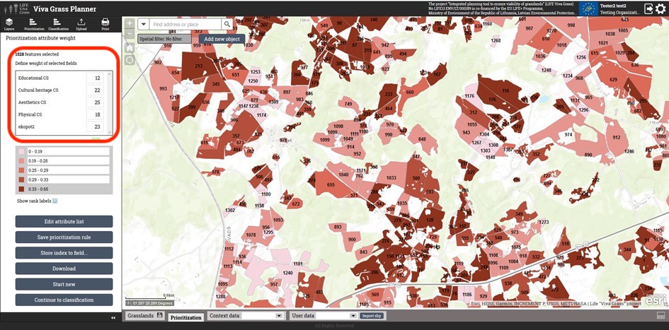
Figure 6.11. Weighting the criteria in Viva Grass Planner. The dark red areas show grasslands that correspond best to the selected criteria.
Classification is an arrangement of data based on selected attributes and can be done both based on performed prioritization and stand alone. To perform classification certain level GIS skills are needed, as it is defined by writing an expression in SQL syntax (Fig.6.12). User have to know the data structure as well.
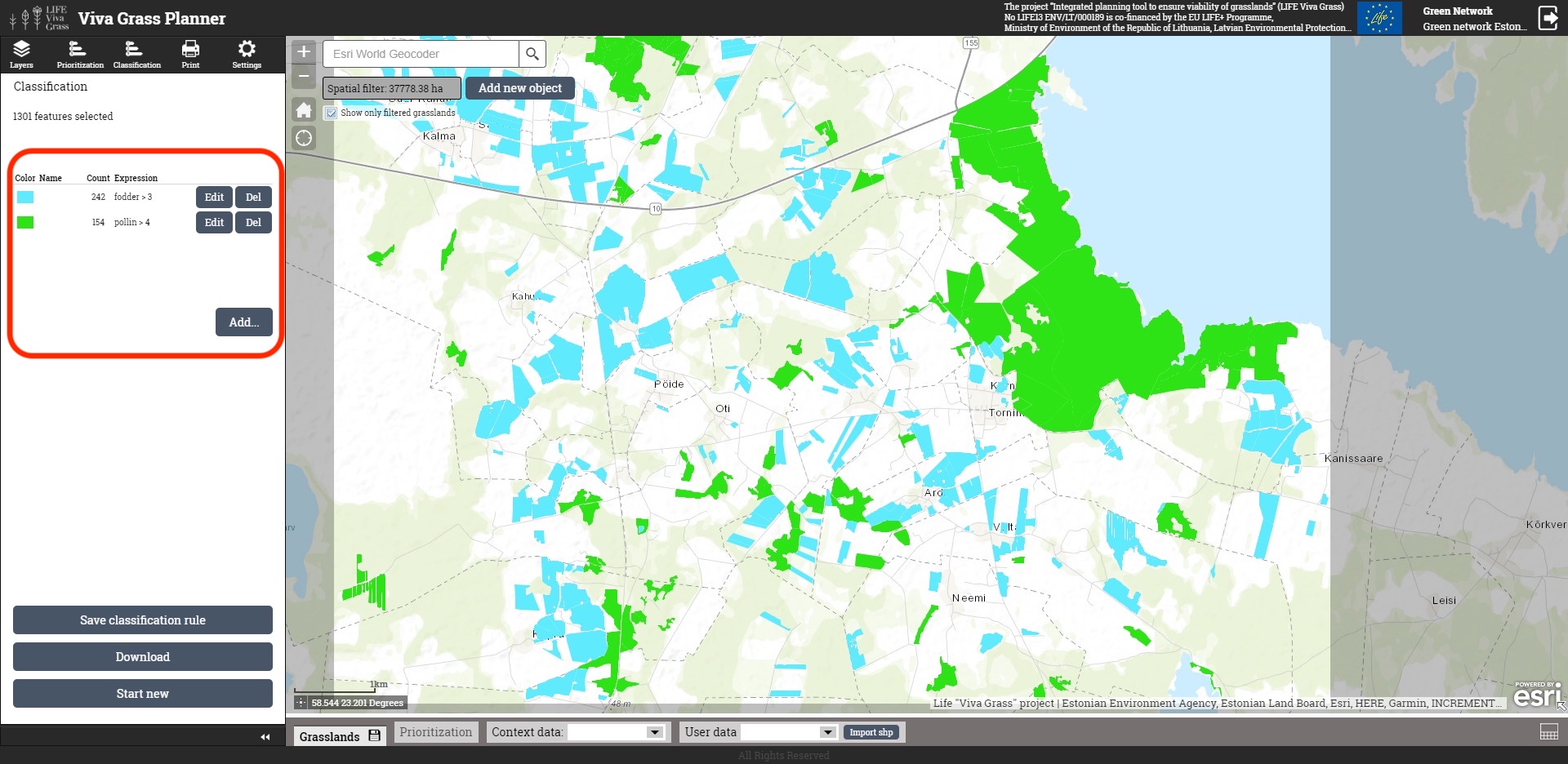
Figure 6.12. Classification in “Viva Grass Planner”. The user can determine the classification rules. The example shows grasslands where fodder provision is higher than 3 (blue areas) and grasslands where pollination provision is higher than 4 (green areas).
To present how to use Viva Grass Planner we have developed several applications of its full functionality addressed at certain objectives of LIFE Viva Grass project. One example is Landscape planning decision support, where according to certain expert developed criteria (Table 6. 1) prioritization and classification of farmland is calculated, subsequent order and intensity of landscape management practices are suggested. The workflow of Landscape management decision support is presented in Figure 6.13.

Table 6.1. Criteria identified and mapped for Landscape planning module
| Criteria | Type | Description |
| Physical and experiential interactions | Cultural ES | Vicinity to recreational objects and territories |
| Educational value | Cultural ES | Vicinity to educational objects and territories |
| Cultural heritage value | Cultural ES | Vicinity to cultural heritage objects and territories |
| Landscape aesthetics value | Cultural ES | Selected landscape features (openness of landscape, relief undulation, vicinity to water bodies and streams, character of land use and character of surrounding land use |
| Ecological value | Aggregated ES values | Average value of ES in “Habitats” bundle |
| Risk of farmland abandonment | Composite indicator | Agro-ecological qualities of farmland, vicinity to farms, roads and settlements |
| Risk of Hogweed Sosnowsky invasion | Composite indicator | Vicinity to invaded sites |
To ensure quality of performed analysis data editing and additional data upload is provided. User are able to edit and store underlying natural conditions of selected field in case there are more precise information available. The calculations of ES supply potential and interactions among ES are recalculated and updated by the “Viva Grass Tool” and further stored in user account.
Default features of place search to navigate map and choosing of defined background maps as well possibility to use custom background map and upload custom data as context layer using WMS are available in “Viva Grass Planner”.
Suggested reading:
Bullock, J., Jefferson, R., Blackstock, T., Pakeman, R., Emmett, B., Pywell, R., Grime, J., Silvertown, J. 2011. Semi-natural grasslands. [UK National Ecosystem Assessment. Understanding nature’s value to society. Technical Report.]UNEP-WCMC, Cambridge. pp. [In English]
Dengler, J., Rūsiņa, S., 2012. Database Dry Grasslands in the Nordic and Baltic Region. Biodiversity & Ecology 4: 319-320. http://dx.doi.org/10.7809/b-e.00114 https://doi.org/10.7809/b-e.00114
Depellegrin, D., Pereira, P., Misiunė, I., Egarter-Vigl, L., 2016. Mapping ecosystem services potential in Lithuania. International Journal of Sustainable Development & World Ecology 23 (5): 441-455. http://dx.doi.org/10.1080/13504509.2016.1146176 https://doi.org/10.1080/13504509.2016.1146176
Dunford, R., Harrison, P., Smith, A., Dick, J., Barton, D., Martin-Lopez, B., Kelemen, E., Jacobs, S., Saarikoski, H., Turkelboom, F., Verheyden, W., Hauck, J., Antunes, P., Aszalós, R., Badea, O., Baró, F., Berry, P., Carvalho, L., Conte, G., Czúcz, B., Blanco, G., Howard, D., Giuca, R., Gomez-Baggethun, E., Grizetti, B., Izakovicova, Z., Kopperoinen, L., Langemeyer, J., Luque, S., Lapola, D., Martinez-Pastur, G., Mukhopadhyay, R., Roy, S., Niemelä, J., Norton, L., Ochieng, J., Odee, D., Palomo, I., Pinho, P., Priess, J., Rusch, G., Saarela, S., Santos, R., der Wal, J., Vadineanu, A., Vári, Á., Woods, H., Yli-Pelkonen, V. 2017. Integrating methods for ecosystem service assessment: Experiences from real world situations. Ecosystem Services: https://doi.org/10.1016/j.ecoser.2017.10.014
Grêt-Regamey, A,, Weibel, B., Kienast, F., Rabe, S., Zulian, G., 2015. A tiered approach for mapping ecosystem services. Ecosystem Services 13: 16-27. https://doi.org/10.1016/j.ecoser.2014.10.008
Smith, A., Harrison, P., Soba, M., Archaux, F., Blicharska, M., Egoh, B., Erős, T., Domenech, N., György, Á., Haines-Young, R., Li, S., Lommelen, E., Meiresonne, L., Ayala, L., Mononen, L., Simpson, G., Stange, E., Turkelboom, F., Uiterwijk, M., Veerkamp, C., de Echeverria, V. 2017. How natural capital delivers ecosystem services: A typology derived from a systematic review. Ecosystem Services 26: 111-126. https://doi.org/10.1016/j.ecoser.2017.06.006
Soukup, T., Feranec, J., Hazeu, G., Jaffrain, G,, Jindrova, M., Kopecky, M., Orlitova, E., 2016. Chapter 11 CORINE Land Cover 2000 (CLC2000): Analysis and Assessment. [European Landscape Dynamics.]. pp. http://dx.doi.org/10.1201/9781315372860-12
Vinogradovs, I,, Nikodemus, O., Elferts, D., Brūmelis, G., 2018. Assessment of site-specific drivers of farmland abandonment in mosaic-type landscapes: A case study in Vidzeme, Latvia. Agriculture, Ecosystems & Environment 253: 113-121. http://dx.doi.org/10.1016/j.agee.2017.10.016 https://doi.org/10.1016/j.agee.2017.10.016
Walz, U., Syrbe, R., Grunewald, K., 2017. Where to map? In: Burkhard B, Maes J (Ed.)[Mapping Ecosystem Services.]Pensoft Publishers, Sofia, Bulgaria. 374 pp. [In English]